
R: Think Bayes Locomotive Problem - Posterior probabilities for different priors
In my continued reading of Think Bayes the next problem to tackle is the Locomotive problem which is defined thus:
A railroad numbers its locomotives in order 1..N. One day you see a locomotive with the number 60. Estimate how many loco- motives the railroad has.
The interesting thing about this question is that it initially seems that we don’t have enough information to come up with any sort of answer. However, we can get an estimate if we come up with a prior to work with.
The simplest prior is to assume that there’s one railroad operator with between say 1 and 1000 railroads with an equal probability of each size.
We can then write similar code as with the dice problem to update the prior based on the trains we’ve seen.
First we’ll create a data frame which captures the product of 'number of locomotives' and the observations of locomotives that we’ve seen (in this case we’ve only seen one locomotive with number '60':)
library(dplyr)

possibleValues = 1:1000
observations = c(60)

l = list(value = possibleValues, observation = observations)
df = expand.grid(l)

> df %>% head()
  value observation
1     1          60
2     2          60
3     3          60
4     4          60
5     5          60
6     6          60
Next we want to add a column which represents the probability that the observed locomotive could have come from a particular fleet. If the number of railroads is less than 60 then we have a 0 probability, otherwise we have 1 / numberOfRailroadsInFleet:
prior = 1  / length(possibleValues)
df = df %>% mutate(score = ifelse(value < observation, 0, 1/value))

> df %>% sample_n(10)
     value observation       score
179    179          60 0.005586592
1001  1001          60 0.000999001
400    400          60 0.002500000
438    438          60 0.002283105
667    667          60 0.001499250
661    661          60 0.001512859
284    284          60 0.003521127
233    233          60 0.004291845
917    917          60 0.001090513
173    173          60 0.005780347
To find the probability of each fleet size we write the following code:
weightedDf = df %>%
  group_by(value) %>%
  summarise(aggScore = prior * prod(score)) %>%
  ungroup() %>%
  mutate(weighted = aggScore / sum(aggScore))

> weightedDf %>% sample_n(10)
Source: local data frame [10 x 3]

   value     aggScore     weighted
1    906 1.102650e-06 0.0003909489
2    262 3.812981e-06 0.0013519072
3    994 1.005031e-06 0.0003563377
4    669 1.493275e-06 0.0005294465
5    806 1.239455e-06 0.0004394537
6    673 1.484400e-06 0.0005262997
7    416 2.401445e-06 0.0008514416
8    624 1.600963e-06 0.0005676277
9     40 0.000000e+00 0.0000000000
10   248 4.028230e-06 0.0014282246
Let’s plot the data frame to see how the probability varies for each fleet size:
library(ggplot2)
ggplot(aes(x = value, y = weighted), data = weightedDf) +
  geom_line(color="dark blue")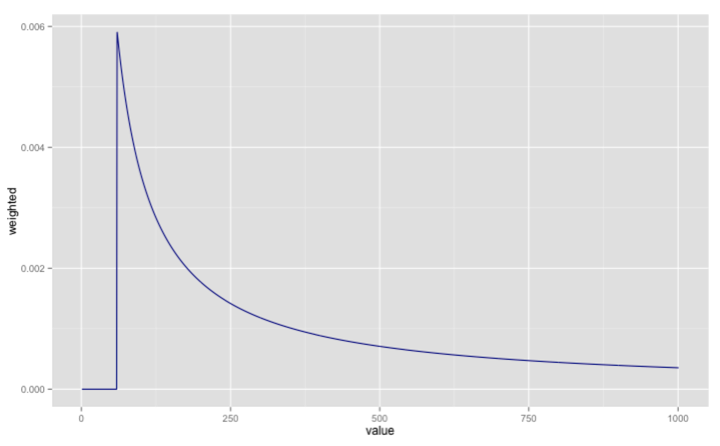
The most likely choice is a fleet size of 60 based on this diagram but an alternative would be to find the mean of the posterior which we can do like so:
> weightedDf %>% mutate(mean = value * weighted) %>% select(mean) %>% sum()
[1] 333.6561
Now let’s create a function with all that code in so we can play around with some different priors and observations:
meanOfPosterior = function(values, observations) {
  l = list(value = values, observation = observations)
  df = expand.grid(l) %>% mutate(score = ifelse(value < observation, 0, 1/value))

  prior = 1  / length(possibleValues)
  weightedDf = df %>%
    group_by(value) %>%
    summarise(aggScore = prior * prod(score)) %>%
    ungroup() %>%
    mutate(weighted = aggScore / sum(aggScore))

  return (weightedDf %>% mutate(mean = value * weighted) %>% select(mean) %>% sum())
}
If we update our observed railroads to have numbers 60, 30 and 90 we’d get the following means of posteriors assuming different priors:
> meanOfPosterior(1:500, c(60, 30, 90))
[1] 151.8496
> meanOfPosterior(1:1000, c(60, 30, 90))
[1] 164.3056
> meanOfPosterior(1:2000, c(60, 30, 90))
[1] 171.3382
At the moment the function assumes that we always want to have a uniform prior i.e. every option has an equal opportunity of being chosen, but we might want to vary the prior to see how different assumptions influence the posterior.
We can refactor the function to take in values & priors instead of calculating the priors in the function:
meanOfPosterior = function(values, priors, observations) {
  priorDf = data.frame(value = values, prior = priors)
  l = list(value = priorDf$value, observation = observations)

  df = merge(expand.grid(l), priorDf, by.x = "value", by.y = "value") %>%
    mutate(score = ifelse(value < observation, 0, 1 / value))

  df %>%
    group_by(value) %>%
    summarise(aggScore = max(prior) * prod(score)) %>%
    ungroup() %>%
    mutate(weighted = aggScore / sum(aggScore)) %>%
    mutate(mean = value * weighted) %>%
    select(mean) %>%
    sum()
}
Now let’s check we get the same posterior means for the uniform priors:
> meanOfPosterior(1:500,  1/length(1:500), c(60, 30, 90))
[1] 151.8496
> meanOfPosterior(1:1000, 1/length(1:1000), c(60, 30, 90))
[1] 164.3056
> meanOfPosterior(1:2000, 1/length(1:2000), c(60, 30, 90))
[1] 171.3382
Now if instead of a uniform prior let’s use a power law one where the assumption is that smaller fleets are more likely:
> meanOfPosterior(1:500,  sapply(1:500,  function(x) x ** -1), c(60, 30, 90))
[1] 130.7085
> meanOfPosterior(1:1000, sapply(1:1000, function(x) x ** -1), c(60, 30, 90))
[1] 133.2752
> meanOfPosterior(1:2000, sapply(1:2000, function(x) x ** -1), c(60, 30, 90))
[1] 133.9975
> meanOfPosterior(1:5000, sapply(1:5000, function(x) x ** -1), c(60, 30, 90))
[1] 134.212
> meanOfPosterior(1:10000, sapply(1:10000, function(x) x ** -1), c(60, 30, 90))
[1] 134.2435
Now we get very similar posterior means which converge on 134 and so that’s our best prediction.
About the author
I'm currently working on short form content at ClickHouse. I publish short 5 minute videos showing how to solve data problems on YouTube @LearnDataWithMark. I previously worked on graph analytics at Neo4j, where I also co-authored the O'Reilly Graph Algorithms Book with Amy Hodler.