
Exploring node2vec - a graph embedding algorithm
In my explorations of graph based machine learning, one algorithm I came across is called node2Vec. The paper describes it as "an algorithmic framework for learning continuous feature representations for nodes in networks".
So what does the algorithm do? From the website:
The node2vec framework learns low-dimensional representations for nodes in a graph by optimizing a neighborhood preserving objective. The objective is flexible, and the algorithm accommodates for various definitions of network neighborhoods by simulating biased random walks.
Running node2Vec
We can try out an implementation of the algorithm by executing the following instructions:
git clone git@github.com:snap-stanford/snap.git
cd snap/examples/node2vec
make
We should end up with an executable file named node2vec:
$ ls -alh node2vec
-rwxr-xr-x  1 markneedham  staff   4.3M 11 May 08:14 node2vec
The download includes the Zachary Karate Club dataset. We can inspect that dataset to see what format of data is expected.
The data lives in graph/karate.edgelist.
The contents of that file are as follows:
cat graph/karate.edgelist | head -n10
1 32
1 22
1 20
1 18
1 14
1 13
1 12
1 11
1 9
1 8
The algorithm is then executed like this:
./node2vec -i:graph/karate.edgelist -o:emb/karate.emb -l:3 -d:24 -p:0.3 -dr -v$ cat emb/karate.emb | head -n5
35 24
31 -0.0419165 0.0751558 0.0777881 -0.13651 -0.0723484 0.131121 -0.133643 0.0329049 0.0891693 0.0898324 0.0177763 -0.0947387 0.0152228 -0.00862188 0.0383254 0.222333 0.117794 0.189328 0.0327467 0.142506 -0.0787722 0.0757344 -0.0127497 -0.0305164
33 -0.105675 0.287809 0.20373 -0.247271 -0.222551 0.257689 -0.258127 0.0844224 0.182316 0.178839 0.0792992 -0.166362 0.114856 0.0422123 0.152787 0.551674 0.332224 0.487846 0.0619851 0.386913 -0.142459 0.173472 0.0184598 -0.100818
34 0.0121748 0.0941794 0.20482 -0.430609 -0.08399 0.293788 -0.322655 0.0704057 0.116873 0.214754 0.138378 -0.207141 -0.0159013 -0.238914 0.037141 0.541439 0.324653 0.458905 0.0216556 0.270057 -0.204671 0.135203 -0.0818273 -0.122353
14 -0.0722407 0.162659 0.111612 -0.20907 -0.11984 0.15896 -0.175391 0.0642012 0.094021 0.125609 0.0465577 -0.131715 0.0683675 -0.0097801 0.0467595 0.340551 0.210111 0.279932 0.0283343 0.231359 -0.112208 0.114253 0.00908989 -0.0907061We now have an embedding for each of our people.
These embeddings aren’t very interesting on their own but we can do interesting things with them. One approach when doing exploratory data analysis is to reduce each of the vectors to 2 dimensions so that we can visualise them more easily.
t-SNE
t-Distributed Stochastic Neighbor Embedding (t-SNE) is a popular technique for doing this and has implementations in many languages. We’ll give the Python version a try, but there is also a Java version if you prefer that.
Once we’ve downloaded that we can create a script containing the following code:
from tsne import tsne
import numpy as np
import pylab

X = np.loadtxt("karate.emb", skiprows=1)
X = np.array([x[1:] for x in X])
Y = tsne(X, 2, 50, 20.0)
pylab.scatter(Y[:, 0], Y[:, 1], 20)
pylab.show()
We load the embeddings from the file we created earlier, making sure to skip the first row since that contains the node id which we aren’t interested in here. If we run the script it will output this chart:
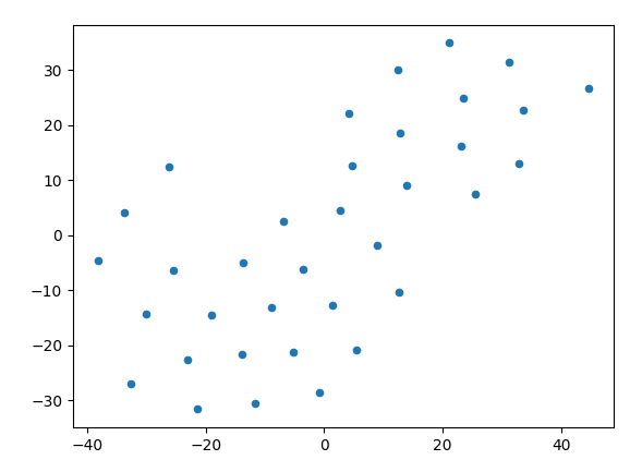
It’s not all that interesting to be honest! This type of visualisation will often reveal a clustering between items but that isn’t the case here.
Now I need to give this a try on a bigger dataset to see if I can find some interesting insights!
About the author
I'm currently working on short form content at ClickHouse. I publish short 5 minute videos showing how to solve data problems on YouTube @LearnDataWithMark. I previously worked on graph analytics at Neo4j, where I also co-authored the O'Reilly Graph Algorithms Book with Amy Hodler.