22 Jun 2021

Apache Pinot: Analysing England's Covid case data

As I mentioned in my last blog post, I’ve been playing around with Apache Pinot, a data store that’s optimised for user facing analytical workloads.

My understanding is that Pinot is a really good fit for datasets where:

The query patterns are of an analytical nature e.g. slicing and dicing on any columns.
We’re ingesting the data in real time from a stream of events. Kenny Bastani has some cool blog posts showing how to do this with Wikipedia and GitHub, and Jackie Jiang showed how to analyse Meetup’s RSVP stream in last week’s Pinot meeetup.

In this blog post I’m going to show how we can use Pinot to analyse Coronavirus case data in England that I downloaded from the UK’s Covid dashboard. This dataset is static, so it would fit in the first category of datasets.

The code used in this post is all included in the github.com/mneedham/pinot-covid-cases GitHub repository.

Setup

We’re going to analyse the dataset using Pinot and its Python driver via a Jupyter notebook. The following Docker Compose config will spin up local instances of Pinot and Jupyter:

docker-compose.yml

version: '3.7'
services:
  pinot:
    image: apachepinot/pinot:0.7.1
    command: "QuickStart -type batch"
    container_name: "pinot-covid-cases"
    volumes:
      - ./config:/config
    ports:
      - "9000:9000"
      - "8000:8000"
  jupyter:
    container_name: "jupyter-covid-cases"
    image: jupyter/scipy-notebook:${JUPYTER_VERSION:-latest}
    volumes:
      - ./notebooks:/home/jovyan
    ports:
      - "8888:8888"

We’ve mounted a directory at /covid on the Pinot container. This directory contains the CSV file that we want to import into Pinot as well as some spec files that we’ll describe later on in this blog post. The contents of the directory are shown below:

Contents of /covid

tree config/covid/cases/
config/covid/cases/
├── job-spec.yml
├── ltla_2021-06-21.csv
├── schema.json
└── table.json

0 directories, 4 files

We can launch the containers by running the following command:

docker-compose up

And then we’re looking for the following lines of output:

Output

...
jupyter-covid-cases    |     To access the notebook, open this file in a browser:
jupyter-covid-cases    |         file:///home/jovyan/.local/share/jupyter/runtime/nbserver-7-open.html
jupyter-covid-cases    |     Or copy and paste one of these URLs:
jupyter-covid-cases    |         http://b3f5460bd961:8888/?token=753baf80a0ac8236a35d12fd0426c85cf476765959513805
jupyter-covid-cases    |      or http://127.0.0.1:8888/?token=753baf80a0ac8236a35d12fd0426c85cf476765959513805
....
pinot-covid-cases | You can always go to http://localhost:9000 to play around in the query console

Dataset

Now that we’re got the infrastructure up and running let’s have a look at the dataset. Below is a sample of the first rows of the CSV file:

Covid cases

areaCode,areaName,areaType,date,age,cases,rollingSum,rollingRate
E06000003,Redcar and Cleveland,ltla,2021-06-16,00_04,0,1,14.1
E06000003,Redcar and Cleveland,ltla,2021-06-16,00_59,15,64,65.9
E06000003,Redcar and Cleveland,ltla,2021-06-16,05_09,0,0,0.0
E06000003,Redcar and Cleveland,ltla,2021-06-16,10_14,1,3,38.1
E06000003,Redcar and Cleveland,ltla,2021-06-16,15_19,1,6,85.6
E06000003,Redcar and Cleveland,ltla,2021-06-16,20_24,2,12,167.6
E06000003,Redcar and Cleveland,ltla,2021-06-16,25_29,2,12,145.4
E06000003,Redcar and Cleveland,ltla,2021-06-16,30_34,2,3,36.6
E06000003,Redcar and Cleveland,ltla,2021-06-16,35_39,2,7,92.1

For each area we have the number of cases per day for each age group.

Before we import this CSV file into Pinot we need to decide which fields we’re going to import and the type of each field. Pinot has three field types:

Dimension - Attributes about the data. We will split the data on these columns and they’ll be used in the selection, filter, and group-by parts of the query.
Date Time - Time stamp for the data. We will filter or group by these columns.
Metric - Measurements. We will aggregate by these columns.

We’ll map our fields as shown below:

Dimension Date Time Metric

Dimension	Date Time	Metric
`areaName`, `areaCode`, `age`	`date`	`cases`

areaName, areaCode, age

date

cases

Create Table

Now we’re going to create a Pinot table to store the data from our CSV file. First, we need to create a schema config, as shown below:

schema.json

{
  "schemaName": "cases",
  "dimensionFieldSpecs": [
    {
      "name": "areaCode",
      "dataType": "STRING"
    },
    {
      "name": "areaName",
      "dataType": "STRING"
    },
    {
      "name": "age",
      "dataType": "STRING"
    }
  ],
  "metricFieldSpecs": [
    {
      "name": "cases",
      "dataType": "INT"
    }
  ],
  "dateTimeFieldSpecs": [{
    "name": "date",
    "dataType": "STRING",
    "format" : "1:DAYS:SIMPLE_DATE_FORMAT:yyyy-MM-dd",
    "granularity": "1:DAYS"
  }]
}

You can find a list of supported data types in the Pinot documentation. Since Pinot doesn’t have a DATETIME type, we need to provide a string or number and indicate its format so that Pinot can convert it into an appropriate format when applying operations against that field.

Once we’ve created the schema config, next up we need to create a table config.

table.json

{
    "tableName": "cases",
    "tableType": "OFFLINE",
    "segmentsConfig": {
      "replication": 1,
      "timeColumnName": "date",
      "timeType": "DAYS",
      "retentionTimeUnit": "DAYS",
      "retentionTimeValue": 365
    },
    "tenants": {
      "broker":"DefaultTenant",
      "server":"DefaultTenant"
    },
    "tableIndexConfig": {
      "loadMode": "MMAP"
    },
    "ingestionConfig": {
      "batchIngestionConfig": {
        "segmentIngestionType": "APPEND",
        "segmentIngestionFrequency": "DAILY"
      }
    },
    "metadata": {}
  }

The table type can be either OFFLINE (for batch ingestion of data) or REALTIME (for streamed ingestion of data).

docker exec -it pinot-covid-cases bin/pinot-admin.sh AddTable \
  -tableConfigFile /config/covid/cases/table.json \
  -schemaFile /config/covid/cases/schema.json -exec

Output

Executing command: AddTable -tableConfigFile /config/covid/cases/table.json -schemaFile /config/covid/cases/schema.json -controllerProtocol http -controllerHost 192.168.96.2 -controllerPort 9000 -exec
Sending request: http://192.168.96.2:9000/schemas to controller: a03d8fd1626e, version: Unknown
{"status":"Table cases_OFFLINE succesfully added"}

The message indicates that a table with the name cases_OFFLINE has been created, but we will be able to query it using the cases name.

Import CSV file

Now that we’ve created our table it’s time to import our CSV file. To do that we’ll need to create an ingestion job spec. An ingestion job spec for our Covid cases CSV file is shown below:

job-spec.yml

executionFrameworkSpec:
  name: 'standalone'
  segmentGenerationJobRunnerClassName: 'org.apache.pinot.plugin.ingestion.batch.standalone.SegmentGenerationJobRunner'
  segmentTarPushJobRunnerClassName: 'org.apache.pinot.plugin.ingestion.batch.standalone.SegmentTarPushJobRunner'
  segmentUriPushJobRunnerClassName: 'org.apache.pinot.plugin.ingestion.batch.standalone.SegmentUriPushJobRunner'
jobType: SegmentCreationAndTarPush
inputDirURI: '/config/covid/cases'
includeFileNamePattern: 'glob:**/*.csv'
outputDirURI: '/opt/pinot/data/cases/segments/'
overwriteOutput: true
pinotFSSpecs:
  - scheme: file
    className: org.apache.pinot.spi.filesystem.LocalPinotFS
recordReaderSpec:
  dataFormat: 'csv'
  className: 'org.apache.pinot.plugin.inputformat.csv.CSVRecordReader'
  configClassName: 'org.apache.pinot.plugin.inputformat.csv.CSVRecordReaderConfig'
tableSpec:
  tableName: 'cases'
pinotClusterSpecs:
  - controllerURI: 'http://localhost:9000'

tableSpec.tableName should match the table name that we used in the table spec and inputDirURI refers to the directory that we mounted when launching the Pinot Docker container.

We can run the ingestion job by running the following command:

docker exec -it pinot-covid-cases bin/pinot-admin.sh LaunchDataIngestionJob \
    -jobSpecFile /config/covid/cases/job-spec.yml

Output

Start pushing segments: [/opt/pinot/data/cases/segments/cases_OFFLINE_2020-01-30_2021-06-16_0.tar.gz]... to locations: [org.apache.pinot.spi.ingestion.batch.spec.PinotClusterSpec@7c214cc0] for table cases
Pushing segment: cases_OFFLINE_2020-01-30_2021-06-16_0 to location: http://localhost:9000 for table cases
Sending request: http://localhost:9000/v2/segments?tableName=cases to controller: a03d8fd1626e, version: Unknown
Response for pushing table cases segment cases_OFFLINE_2020-01-30_2021-06-16_0 to location http://localhost:9000 - 200: {"status":"Successfully uploaded segment: cases_OFFLINE_2020-01-30_2021-06-16_0 of table: cases"}

Querying Pinot

We’re going to query Pinot via a Jupyter notebook, which is available at http://localhost:8888/notebooks/Explore.ipynb if you’re playing along. You can also find the notebook at github.com/mneedham/pinot-covid-cases/blob/main/notebooks/Explore.ipynb.

First we need to install the Pinot Python driver:

pip install pinotdb

We’re going to visualise the results of our queries using matplotlib, so let’s import that library and pinotdb:

from pinotdb import connect
import pandas as pd
pd.options.plotting.backend = "matplotlib"
import matplotlib.pyplot as plt

plt.style.use('fivethirtyeight')

Next we’ll create a connection to the database and run a query that counts the number of rows to make sure that everything’s working:

conn = connect(host='pinot-covid-cases', port=8000, path='/query/sql', scheme='http')

curs = conn.cursor()
curs.execute("""
SELECT count(*)
FROM cases
""")
for row in curs:
    print(row)

Output

[3234594]

So far so good!

Now let’s write some more Pinoty (I’m sure that’s not a word!) queries. First up, which areas have had the most cases:

curs.execute("""
SELECT areaName, sum(cases) AS totalCases
FROM cases
GROUP BY areaName
ORDER BY totalCases DESC
LIMIT 10
""")

df_by_area = pd.DataFrame(curs, columns=["areaName", "numberOfCases"])
df_by_area

Table 1. Areas with the most Covid cases
areaName	numberOfCases
Birmingham	210443.0
Leeds	134366.0
Manchester	118021.0
Bradford	104650.0
Liverpool	100411.0
Sheffield	90652.0
County Durham	79115.0
Leicester	77274.0
Kirklees	74164.0
Newham	72602.0

We can then create a matplotlib visualisation of that data using the code below:

ax = df_by_area.plot(
    kind="bar",
    x="areaName",
    y="numberOfCases",
    legend=None,
    figsize=(10, 5)
)

ax.set(xlabel="Area Name", ylabel="Number of cases")
ax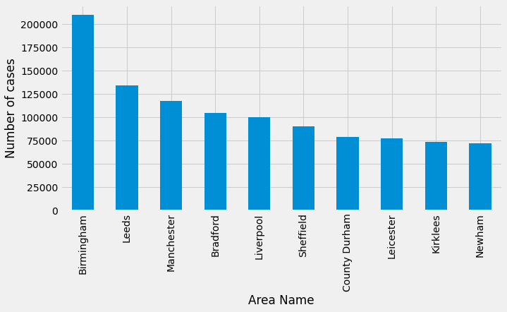

Figure 1. Top areas for Coronavirus cases

It’s a bit tricky to interpret the results of this query because it’s not really telling us that the most cases have been in the midlands and north of England. Rather the break down of the local areas in that part of the country doesn’t seem to be as granular as in London, for example.

Talking of London, for our next query we’ll filter the data to only return rows for the areaName of Sutton, and return the total number of cases by age group:

area_name="Sutton"
curs.execute(f"""
SELECT age, sum(cases) as totalCases
from cases
WHERE areaName = '{area_name}'
GROUP BY age
ORDER BY totalCases DESC
limit 50
""")

df_by_area = pd.DataFrame(curs, columns=["age", "numberOfCases"])
df_by_area

ax = df_by_area.plot(
    kind="bar",
    x="age",
    y="numberOfCases",
    legend=None,
    figsize=(10, 5)
)

ax.set(xlabel="Age Group", ylabel="Number of cases")
ax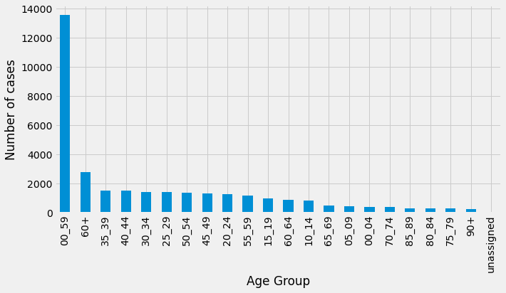

Figure 2. Coronavirus cases by age group in Sutton

From these results we can see that the number of cases are being double booked - once as a fine grained age range (e.g. 35-39 or 80-84) and once as a coarse grained age range (0-59 or 60+). Let’s now have a look at the number of cases in Sutton going back to March 2020 excluding the coarse grained age groups:

area_name="Sutton"
curs.execute(f"""
SELECT "date", sum(cases) AS totalCases
FROM cases
WHERE areaName = '{area_name}' AND age not in ('00_59', '60+')
GROUP BY "date"
ORDER BY "date"
LIMIT 1000
""")

df_by_area = pd.DataFrame(curs, columns=["date", "numberOfCases"])

ax = df_by_area.plot(
    kind="line",
    x="date",
    y="numberOfCases",
    legend=None,
    figsize=(10, 5),
    linewidth=1
)

ax.set(xlabel="Area Name", ylabel="Number of cases")
ax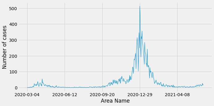

Figure 3. Coronavirus cases per day in Sutton

The most cases happened at the end of December 2020/beginning of January 2020, with the peak on 29th December.

In Summary

I appreciate that we’ve only brushed the surface of what Pinot can do in this blog post, but I had to start somewhere and it’s been a fun tool to play with.

I think my next dataset needs to have more columns per row and preferably have more than one metrics column. I also need to learn more about indexing and in particular the Star-Tree Index that the company behind Pinot is named after.

I should also say that I found the Pinot Community Slack really helpful for getting up to speed. Special thanks to Neha Pawar and Mayank Shrivastava for answering my questions!

About the author

I'm currently working on short form content at ClickHouse. I publish short 5 minute videos showing how to solve data problems on YouTube @LearnDataWithMark. I previously worked on graph analytics at Neo4j, where I also co-authored the O'Reilly Graph Algorithms Book with Amy Hodler.