28 Jul 2023

Apache Pinot: Experimenting with the StarTree Index

My colleagues Sandeep Dabade and Kulbir Nijjer recently wrote a three part blog post series about the StarTree index, an Apache Pinot indexing technique that dynamically builds a tree structure to maintain aggregates across a group of dimensions. I’ve not used this index before and wanted to give it a try and in this blog post, I’ll share what I learned.

I’ve put all the code in the startreedata/pinot-recipes GitHub repository in case you want to try it out yourself.

Setup

Let’s start by cloning the repository and navigating to the StarTree index recipe:

git clone git@github.com:startreedata/pinot-recipes.git
cd pinot-recipes/recipes/startree-index

We can then spin up Apache Pinot and friends using Docker Compose:

docker compose up

Data Generator

I’ve created a data generator that simulates website traffic. It used the Faker library, so make sure that you install that:

pip install faker

Now let’s run it and have a look at one of the generated messages:

python datagen.py 2>/dev/null | head -n1 | jq

Output

{
  "ts": 1690559577897,
  "userID": "a56717ef",
  "timeSpent": 622,
  "pageID": "page032",
  "country": "Saint Lucia",
  "deviceType": "Mobile",
  "deviceBrand": "Dell",
  "deviceModel": "Google Pixel 6",
  "browserType": "Chrome",
  "browserVersion": "92.0.4515.159",
  "locale": "zh_CN"
}

We have a variety of information about the page visit, including details about the device and browser used. We’re going to ingest that data into Apache Kafka, so let’s first create a topic:

rpk topic create -p 5 webtraffic

And now let’s ingest data into that topic:

python datagen.py 2>/dev/null |
jq -cr --arg sep ø '[.userID, tostring] | join($sep)' |
kcat -P -b localhost:9092 -t webtraffic -Kø

Apache Pinot Tables

We’re going to create several tables in Apache Pinot to explore this dataset:

webtraffic: No indexes
webtraffic_inverted: Inverted index on country, browserType, and deviceBrand. The config looks like this:

{
    "tableIndexConfig": {
        "invertedIndexColumns": [
            "country", "browserType", "deviceBrand"
        ]
    }
}

webtraffic_stree: StarTree index splitting on country, browserType, and deviceBrand, aggregating COUNT(*), SUM(timeSpent), and AVG(timeSpent). The config looks like this:

{
    "tableIndexConfig": {
        "starTreeIndexConfigs": [
          {
            "dimensionsSplitOrder": [
              "country",
              "browserType",
              "deviceBrand"
            ],
            "skipStarNodeCreationForDimensions": [],
            "functionColumnPairs": [
              "COUNT__*",
              "SUM__timeSpent",
              "AVG__timeSpent"
            ],
            "maxLeafRecords": 10000
          }
        ]
    }
}

Queries

Once I’d created the tables, I waited for the data generator to get a bunch of data ingested. I stopped the generator once it had got to 175 million rows, which isn’t big data, but should be enough records for us to see how the indexes work.

From my understanding, the StarTree index should work well when we have to do filtering and then aggregation of data. An inverted index is also good at filtering, so that configuration will serve as a useful comparison.

I came up with the following queries to kick the tyres:

Aggregating time spent by country: This is a pure aggregation query, so the inverted index shouldn’t help at all.

select country, sum(timeSpent) AS totalTime
from webtraffic
group by country
order by totalTime DESC
limit 10

Filtering by country and aggregating by count: This query filters by the country column and then counts the records returned (2.2 million) by browser type. We’d expect the inverted index to do better than the one with no indexes, but StarTree’s pre indexing should give it the edge.

select browserType, count(*)
from webtraffic
WHERE country IN ('Germany', 'United Kingdom', 'Spain')
GROUP BY browserType
limit 10

Comparing query performance

I ran these queries a few times in the Pinot UI to see how well they performed, but I figured that I should probably use a load generator to get more consistent results. I’m going to use a Python performance testing tool called Locust to do this.

Keep in mind that I’m doing all these experiments on my laptop, so you can undoubtedly achieve better results if you use a cluster and don’t have the load-testing tool running on the same machine. But for my purposes of doing something quick and dirty to understand how these indexes help with query performance, this setup does the job.

After installing Locust:

pip install locust

I created a locustfile.py that looked like this:

locustfile.py

from locust import FastHttpUser, task

import requests
import random

query1 = """
select country, sum(timeSpent) AS totalTime
from webtraffic
group by country
order by totalTime DESC
limit 10
"""

query2 = """
select browserType, count(*)
from webtraffic
WHERE country IN ('Germany', 'United Kingdom', 'Spain')
GROUP BY browserType
limit 10
"""

class PinotUser(FastHttpUser):

    @task
    def run_q1(self):
        with super().rest("POST", "/query/sql", json={"sql": query3}, name="Web Traffic (StarTree)") as r:
            if r.status_code == requests.codes.ok:
                # print("/query/sql   - q1" + ': success (200)')
                pass
            elif r.status_code == 0:
                print("/query/sql - q1" + ': success (0)')
                r.success()
            else:
                print("/query/sql - q1" + ': failure (' + str(r.status_code) + ')')
                r.failure(r.status_code)

I then ran the load generator configured to simulate a single user executing the query lots of times:

locust --host http://localhost:8099  \
  --autostart \
  -u 1 \ (1)
  --run-time 1m \
  --autoquit 5 (2)

1	Simulate having 1 user.
2	Exit 5 seconds after the test has been completed.

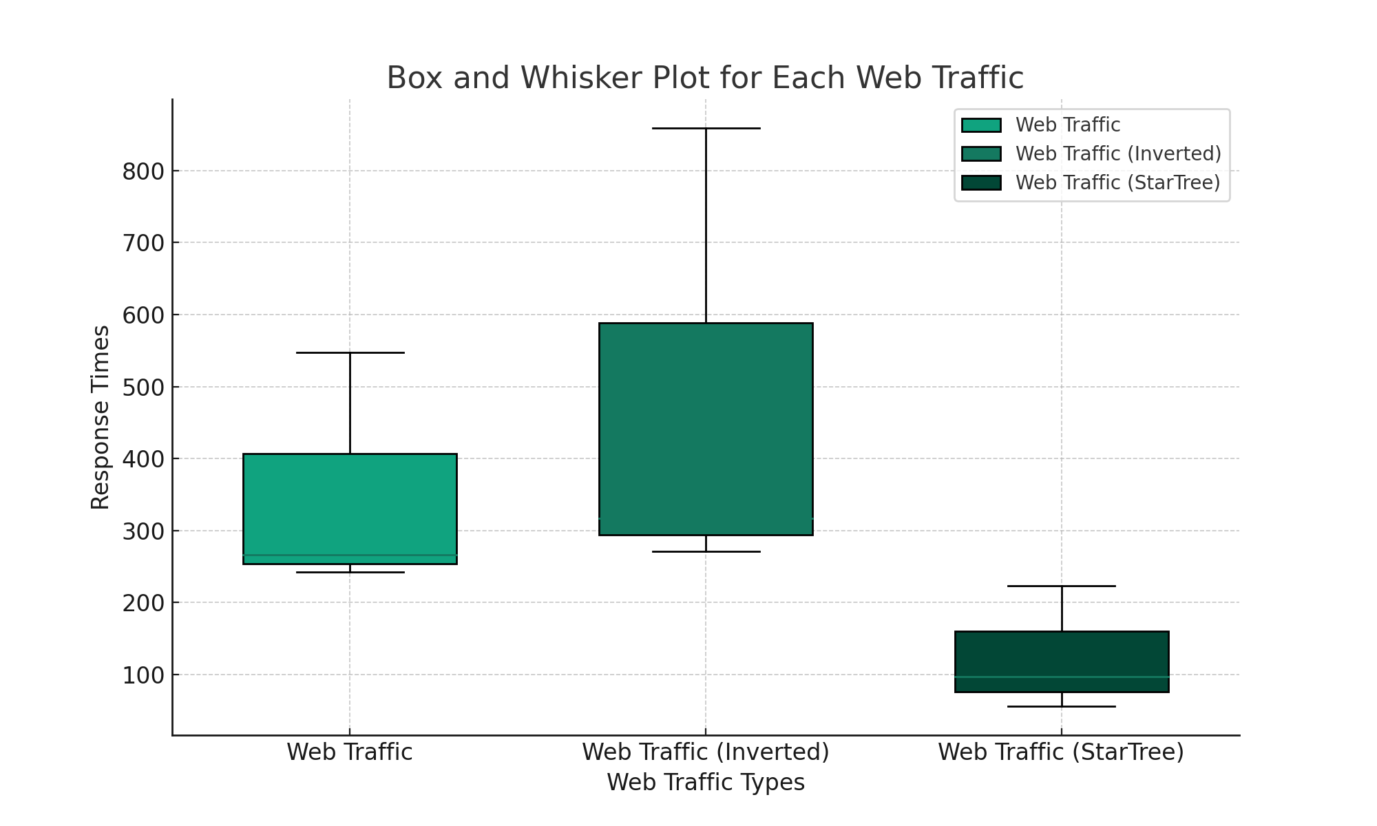
I ran this script 3 times for each query, manually updating the script to run each query against each table. I then collected the results that were printed to the console into the tables shown below:

Table 1. Aggregating time spent by country
Name	# reqs	Avg	Min	Max	Med	req/s
Web Traffic	223	266	242	547	250	3.74
Web Traffic (Inverted)	187	317	271	859	300	3.14
Web Traffic (StarTree)	610	97	56	223	98	10.19

I asked ChatGPT to create a box and whisker plot of this data, which is shown below:

Figure 1. Box and whisker chart - aggregate time spent by country query

Table 2. Filtering by country and aggregating by count
Name	# reqs	Avg	Min	Max	Med	req/s
Web Traffic Filter	501	118	114	706	120	8.38
Web Traffic Filter (Inverted)	2741	20	18	766	20	45.79
Web Traffic Filter (StarTree)	7288	7	6	158	7	121.73

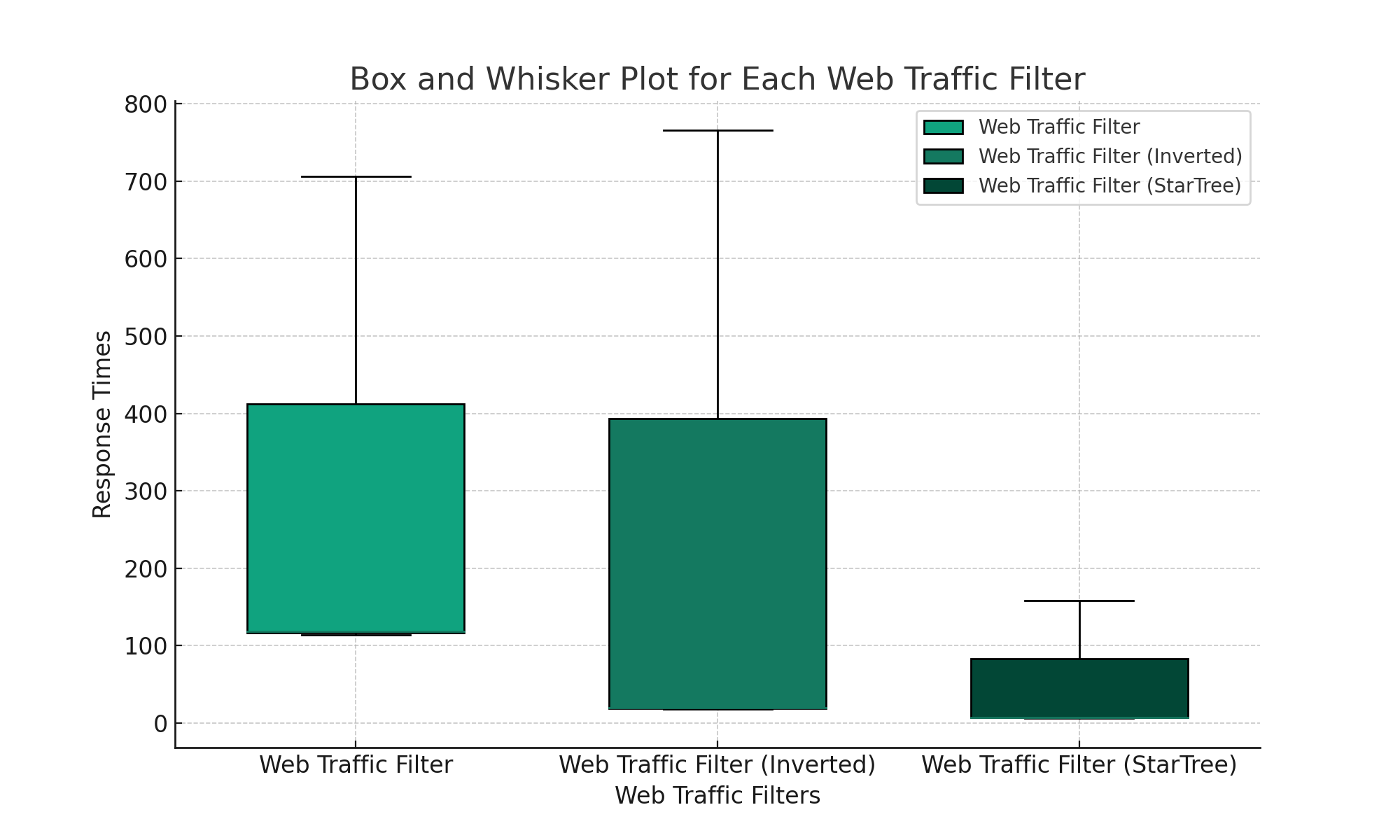
Figure 2. Box and whisker chart - aggregate time spent by country query

From these results, we can see that the StarTree index does best on both queries, but there’s not much in it on the filtering query. I still haven’t quite worked out how many records you need in the aggregation step to see a noticeable improvement compared to doing normal aggregation.

A fun experiment though and I’ll have to do some more of these!

About the author

I'm currently working on short form content at ClickHouse. I publish short 5 minute videos showing how to solve data problems on YouTube @LearnDataWithMark. I previously worked on graph analytics at Neo4j, where I also co-authored the O'Reilly Graph Algorithms Book with Amy Hodler.