14 Sep 2023

FAISS: Exploring Approximate Nearest Neighbours Cell Probe Methods

I’ve been learning about vector search in recent weeks and I came across FaceBook’s FAISS library. I wanted to learn the simplest way to do approximate nearest neighbours, and that’s what we’ll be exploring in this blog post.

I’ve created a video showing how to do this on my YouTube channel, Learn Data with Mark, so if you prefer to consume content through that medium, I’ve embedded it below:

You can also find all the code at the ANN-Tutorial.ipynb notebook.

First things first, let’s install some libraries:

pip install faiss-cpu pandas numpy

We’ll be using the following imports:

import faiss
import copy
import numpy as np
import pandas as pd
import plotly.graph_objects as go
from plotly_functions import generate_distinct_colors, zoom_in, create_plot, plot_points

plotly_functions contains a bunch of helper functions for making it easier to create charts with plot.ly.

Create vectors

We’re going to create 10,000 2D vectors to keep things simple.

dimensions = 2
number_of_vectors = 10_000
vectors = np.random.random((number_of_vectors, dimensions)).astype(np.float32)

Next, let’s create a search vector, whose neighbours we’re going to find:

search_vector = np.array([[0.5, 0.5]])

Creating a cell probe index

The simplest version of approximate nearest neighbours in FAISS is to use one of the cell probe methods. These methods partition the vector space into a configurable number of cells using the K-means algorithm. When we look for our search vector’s neighbours, it’s going to find the centroid closest to the search vector and then search for all the other vectors that belong to the same cell as that centroid.

We can create a cell probe index like this:

cells = 10
quantizer = faiss.IndexFlatL2(dimensions)
index = faiss.IndexIVFFlat(quantizer, dimensions, cells)

To create the centroids, we need to call the train function:

index.train(vectors)

We can then find the centroids by querying the quantizer

centroids = index.quantizer.reconstruct_n(0, index.nlist)
centroids

Output

array([[0.8503718 , 0.46587527],
       [0.14201212, 0.80757564],
       [0.831061  , 0.82165515],
       [0.5756452 , 0.54481953],
       [0.5543639 , 0.1812697 ],
       [0.84584594, 0.16083847],
       [0.259557  , 0.5097532 ],
       [0.23731372, 0.12491277],
       [0.47171366, 0.8513159 ],
       [0.08305518, 0.30214617]], dtype=float32)

Visualising cells and centroids

Next, let’s look at how we can visualise how the vector space has been split. We can work out which cell each vector has been assigned to by calling the search function on the quantizer:

_, cell_ids = index.quantizer.search(vectors, k=1)
cell_ids = cell_ids.flatten()
cell_ids[:10]

Output

array([0, 4, 3, 1, 1, 8, 9, 4, 0, 9])

So far so good. Now let’s create a plot visualising that:

color_map = generate_distinct_colors(index.nlist) (1)

fig_cells = create_plot()

unique_ids = np.unique(cell_ids)
for uid in unique_ids: (2)
  mask = (cell_ids == uid)
  masked_vectors = vectors[mask]
  plot_points(fig_cells, masked_vectors, color_map[uid], "Cell {}".format(uid), size=6) (3)

plot_points(fig_cells, centroids, symbol="diamond-tall", color="black", size=15, showlegend=False) (4)
plot_points(fig_cells, search_vector, symbol="x", color="black", size=15, label="Search Vector") (5)

fig_cells

1	Get a list of unique colours for each cell
2	Iterate over the cells
3	Plot each vector with the colour assigned to its cell id
4	Plot the centroid of each cell
5	Plot the search vector

The resulting visualisation is shown below:

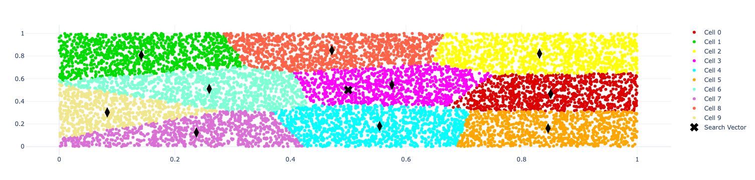
Figure 1. Vectors and their cell assignments

When creating the index, we need to specify how many partitions (or cells) we want to divide the vector space into.

Searching for our vector

It’s time to search for our vector. We’ll start by adding the vectors to the index:

index.add(vectors)

And now let’s call the search function:

distances, indices = index.search(search_vector, k=10)

df_ann = pd.DataFrame({
  "id": indices[0],
  "vector": [vectors[id] for id in indices[0]],
  "distance": distances[0],
})
df_ann

Table 1. df_ann
	id	vector	distance
0	5212	[0.49697843 0.49814904]	1.2555936e-05
1	8799	[0.49676004 0.5018034 ]	1.3749583e-05
2	1553	[0.50321424 0.49744475]	1.6860648e-05
3	8457	[0.4928198 0.50775784]	0.00011173959
4	9626	[0.5133499 0.50718963]	0.00022991038
5	9408	[0.49085045 0.512838 ]	0.00024852867
6	8177	[0.48392993 0.49651426]	0.00027039746
7	1959	[0.502832 0.51659614]	0.000283452
8	5451	[0.48319575 0.5047141 ]	0.00030460523
9	4580	[0.51834625 0.49356925]	0.00037793937

We’ve got a bunch of vectors that are very close to the search vector. When we ran the search function, FAISS first looked for the cell in which it needed to search. We can figure out which cell it used by asking the quantizer:

_, search_vectors_cell_ids = index.quantizer.search(search_vector, k=1)
unique_searched_ids = search_vectors_cell_ids[0]
unique_searched_ids

Output

array([3])

So the nearest cell to 0.5, 0.5 is the one with index 3. If we wanted to find the nearest two cells, we could pass in a different k value.

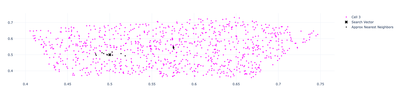
We can visualise the nearest neighbours that it’s found by running the following code:

fig_search = create_plot()

for uid in unique_searched_ids: (1)
  mask = (cell_ids == uid)
  masked_vectors = vectors[mask]
  plot_points(fig_search, masked_vectors, color_map[uid], label="Cell {}".format(uid)) (2)
  plot_points(fig_search, centroids[uid].reshape(1, -1), symbol="diamond-tall", color="black", size=10, label="Centroid for Cell {}".format(uid), showlegend=False) (3)

plot_points(fig_search, points=search_vector, color='black', label="Search Vector", symbol="x", size=10)

ann_vectors = np.array(df_ann["vector"].tolist())
plot_points(fig_search, points=ann_vectors, color='black', label="Approx Nearest Neighbors") (4)

fig_search

1	Iterate over the cells used in the search (i.e. only cell with index=3)
2	Plot the vectors in this cell
3	Plot the centroid for the cell
4	Plot the nearest neighbours

The resulting visualisation is shown below:

Figure 2. Approximate nearest neighbours

Brute Force vs ANN

It looks like ANN has done pretty well, but let’s compare it to the brute force approach where we compare the search vector with every other vector to find its neighbours. We can create a brute force index like this:

brute_force_index = faiss.IndexFlatL2(dimensions)
brute_force_index.add(vectors)

And then search like this:

distances, indices = brute_force_index.search(search_vector, k=10)

pd.DataFrame({
  "id": indices[0],
  "vector": [vectors[id] for id in indices[0]],
  "distance": distances[0],
  "cell": [cell_ids[id] for id in indices[0]]
})

Table 2. Brute Force
	id	vector	distance	cell
0	5212	[0.49697843 0.49814904]	1.2555936e-05	3
1	8799	[0.49676004 0.5018034 ]	1.3749583e-05	3
2	1553	[0.50321424 0.49744475]	1.6860648e-05	3
3	8457	[0.4928198 0.50775784]	0.00011173959	3
4	9626	[0.5133499 0.50718963]	0.00022991038	3
5	9408	[0.49085045 0.512838 ]	0.00024852867	3
6	8177	[0.48392993 0.49651426]	0.00027039746	3
7	1959	[0.502832 0.51659614]	0.000283452	3
8	5451	[0.48319575 0.5047141 ]	0.00030460523	3
9	4580	[0.51834625 0.49356925]	0.00037793937	3

The results are the same as we got with ANN and we can see that all the neighbours belong to cell 3, which was the one used by ANN.

We can actually tweak ANN to search across more than 1 cell by setting the nprobe attribute. For example, if we wanted to search the two closest cells, we would do this:

index.nprobe = 2

And then re-run the search code above. The result for this dataset wouldn’t change since it’s relatively small and has low dimensionality, but with bigger datasets this is a useful thing to play around with.

About the author

I'm currently working on short form content at ClickHouse. I publish short 5 minute videos showing how to solve data problems on YouTube @LearnDataWithMark. I previously worked on graph analytics at Neo4j, where I also co-authored the O'Reilly Graph Algorithms Book with Amy Hodler.